Just like a company traded on the stock market, an income-producing real estate property can be valued based on the sum of the discounted values of its future expected cash flows. This is known as the discounted cash flow (DCF) method of valuation. The method entails first inflating future operating values based on growth assumptions (e.g., tenant lease escalation schedules, operating expense inflation), followed by the discounting of both future estimated net property operating income and net property sale cash flows to a present value based on the transaction’s risk profile.
The discount rate you select to contract the size of the future cash flow amounts should represent the opportunity cost percentage return that a similarly-risky investment alternative would provide you. Choice of discount rate is highly subjective, and there is no verifiable “right” rate to choose, unfortunately. More on discount rate selection can be found here.
An example of DCF-based property valuation follows.
Let’s assume for simplicity that:
- we purchase a property in all cash for $100MM at a 6.2% going-in cap rate ($6.2MM/$100MM),
- there are no acquisition transaction costs,
- there are no capital costs below the NOI line beyond what capital reserves fund,
- we do not reinvest annual cash returns in the property, and
- we sell at the end of Year 4 for $110MM.
This group of assumptions, along with adjusted NOI (net operating income, or income less expenses) values for years 2 through 4, is reflected in the basic projection setup below.
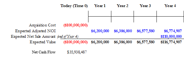
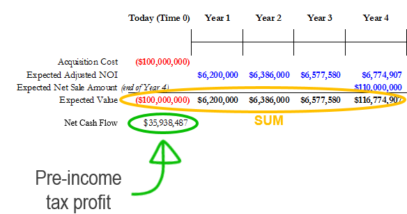
The nominal net cash flow amount (pre-income tax profit) of $35,938,487 (circled in green below, the sum of the values circled in orange below) reflects the growth assumptions and expense inflation assumptions, but if we regard this 35.9MM dollar amount as the net “value created” by the four-year long transaction, it would suggest we have 100% confidence in all of the projected values ending up being what we forecasted them to be.
But the reality is that we can’t knowingly tell a true story about the future any more than the next person can, so if we are honest with ourselves, we admit that we don’t have 100% confidence in the expected values coming to pass as shown on the spreadsheet. As a result, we discount all values (other than the Time 0 value) on a compounded basis at the assumed annual discount rate. We note that some will choose a relatively lower rate for the early years and a relatively higher rate for the late years due to uncertainty increasing the further out we project, but we will assume a constant rate because it all averages out to a constant rate at the end of the day. In the example below, we are using a 7% annual discount rate (shown in blue).
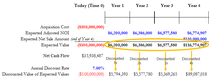
As shown circled in orange above, we take the the nominal expected values in years 1 through 4 and discount them the appropriate number of times. The basic math behind this (which underlies the Present Value, or PV function in Excel) is:
future value / (1+ annual discount rate)^(# of years of discounting)
where the ^ represents the exponent operator. An example of this is the Year 2 expected value of $6,386,000 discounting down to $5,577,780 based on this math: $6,386,000/(1.07)^(2).
Now, as shown below circled in orange, if we sum the discounted values of the expected values, we see that they total $105,828,455. If we were to have added the nominal (undiscounted) expected values (the “Expected Value” line) for years 1 through 4
- $6,200,000
- $6,386,000
- $6,577,580
- $116,774,907
then the total would have been $135,938,487. So the discounting activity has resulted in a reduction of the total perceived value of the future cash flows of the property by approximately $30MM (the difference between $135,938,487 without discounting and $105,828,455 with discounting).
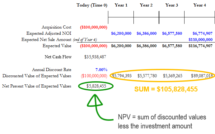
So standing here today, we perceive the property’s present value, to us, based on our own projections of future cash flows and our own discount rate — i.e., its worth — is $105,828,455. The Net Present Value (NPV) of the transaction (with an emphasis on the modifier Net), circled in green above, is $5.8MM, as calculated by deducting our anticipated $100MM acquisition cost from the property’s $105,828,455 present value. Now it’s up to us to decide if this NPV is attractive enough to us, or if we should reduce our offered pricing to increase the NPV further.
Variances in future projection values, discount rates and going-in cap rate requirements across a pool of buyers is what makes bids on properties come in at different values. The spread of the bids will depend on just how widely these amounts and requirements vary.