|
Listen to this post if you prefer
|
There’s sometimes misunderstanding as it relates to cash flow waterfall modeling with mixing up of the terms catch-up, clawback and look-back. To be clear, each is completely its own concept. In this post we will shed some needed light on the look-back mechanism. (We’ve previously addressed catch-up and clawback in separate posts.)
Look-back relates to the use of hurdles as the method for determining which portions of overall property-level equity cash flows should be distributed to each of the JV entities at each of the unique cash flow splitting percentages tied to the distinct tiers in a waterfall (as a refresher, a tier is best thought of as a range of investment performance). For instance, there might be a hurdle that is predicated on the equity achieving a certain IRR or a certain multiple on equity.
Condominium development case study
To teach the concept of the look-back, we’ll use the example of an equity JV that is developing a 30-unit, 5-story residential condominium building.
Assumptions:
- there are 6 units on each of the 5 floors of the building
- all of the units in the building sell for the same price (this is a simplifying assumption made on purpose)
- the units in the project are sold from the bottom up (i.e., Floor 1 sells and closes all its units first, then Floor 2, etc.) (this is also a simplifying assumption made on purpose).
JV waterfall structure
The sponsor-investor joint venture invests $2.079MM in cash equity in aggregate (“dollars in”, split 10% from the sponsor and 90% from the investor), and for “dollars out”, there is a 10% IRR-based Preferred Return distributed to both sponsor and investor (this is Tier 1), after which cash flows are split 50% to the sponsor and 50% to the investor (this is Tier 2). The IRR that is used as the hurdle rate is that of the project.
Understanding the purpose of the look-back
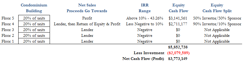
The gross positive cash flow back to equity is $5.85MM, with the net being $3.77MM (gross less invested amount of ~$2.1MM). The project IRR is 43.26%. Given that certain portions of the gross cash flow will be distributed 90%/10% for Tier 1, and other portions will be distributed 50%/50%, the question becomes: how do we know which dollars should be split in each of the specified proportions?
This is the express purpose of the look-back mechanism — to tease out those cash flow dollar amounts that are unique to each Tier in the waterfall so they can be split up appropriately.
How the look-back works
The look-back runs a simple calculation to answer the following question: what would cash flows be IF the negotiated level of return were achieved?
For example, if the negotiated (targeted, not guaranteed!) Preferred Return IRR is 10% to both the investor and the sponsor, we take their aggregate capital invested and compound it at that 10% annual rate (IRR is annual-based) over the term of the investment to solve for what cash flows would be if the project did in fact achieve at least a 10% equity IRR. We compound it at whatever frequency is stated in the JV operating agreement (typically daily, monthly or quarterly) on a cumulative accrual basis, and the result is an absolute amount against which we can make distributions for the purpose of the stated Preferred Return level of distribution.
Where the sale cash flows go and how they impact the IRR and equity multiple
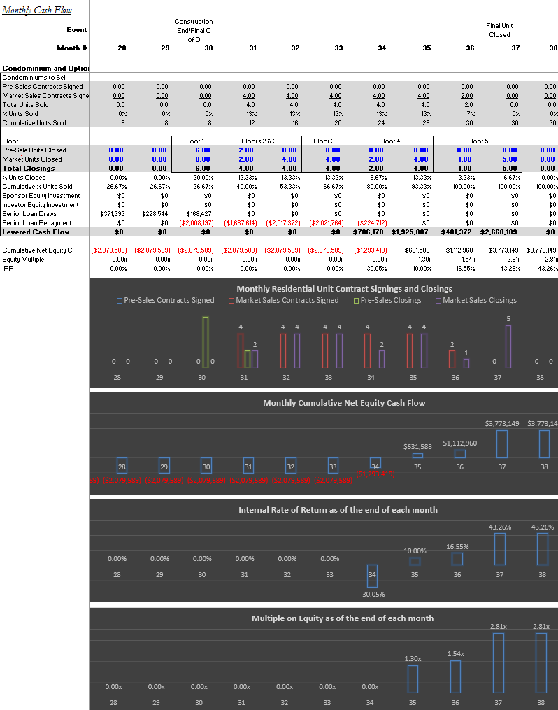
Using the monthly projection below, we can see in months 30-34 that all of the net sales proceeds cash flows coming from Floors 1-3, and some of the cash flows from the net sales proceeds of Floor 4, go towards Senior Loan Repayment. The balance of the units in the property on Foors 4 and 5 all produce cash flows that go exclusively to equity, both for the purpose of returning the capital invested and distributing all profits.
A couple items to note:
- Regarding the third graph below: the IRR has been forced to be zero during those periods in which it is so negative that it’s incalculable (IRR will not produce a result until the first dollar of equity capital has been returned, which in our case does not happen until month 34). If we did not force it to be zero, we would not have been able to graph the series.
- In month 35, the following all occur:
- Cumulative net equity cash flow goes positive (i.e., equity not only breaks even on their $2.079MM investment, but also makes its first dollars of profit)
- the Equity Multiple rises above 1.00x, and
- the IRR goes from negative to positive.
Insights to take away
Using the simplifying assumptions that all units sell for the same price and the building settles units from the bottom up, we can understand the waterfall distribution splits by tying the floors of the property to the equity cash flows. The Floor 4 equity cash flow of $2.711MM ($786,170 in month 34 plus $1,925,007 in month 35) is the exact amount that provides a 10% IRR to the $2.079MM in equity invested over the assumed investment period. This $2.711MM returns the invested capital in full and also distributes profits up through the 10% IRR level.
Floor 5 unit net sales proceeds elevate the IRR from above a 10% IRR to the final project IRR of 43.26%, and are distributed 50%/50%.
We note that in this exact example, look-back accrual mechanics would actually not be needed in your spreadsheet because the exact hurdle rate of 10% is perfectly achieved as of the end of a discrete period (month 35). The odds of this happening are essentially 0%, though, and that’s why the look-back accrual math is present in cash flow waterfall spreadsheets.
To learn about how to compute accruals for all periodic frequencies and solve for distributions in look-back based waterfalls with up to 5 Tiers, buy our Level 3 JV Waterfall Modeling Bootcamp.